Math
Functions
The function specification in JSBSim is a powerful and versatile resource that allows algebraic functions to be defined in a JSBSim configuration file. The function syntax is similar in concept to MathML (Mathematical Markup Language, http://www.w3.org/Math/), but it is simpler and more terse.
A function definition consists of an operation, a value, a table, or a property (which evaluates to a value). The currently supported operations are:
sum(takes n arguments)difference(takes n arguments)product(takes n arguments)quotient(takes 2 arguments)pow(takes 2 arguments)exp(takes 2 arguments)abs(takes n arguments)sin(takes 1 arguments)cos(takes 1 arguments)tan(takes 1 arguments)asin(takes 1 arguments)acos(takes 1 arguments)atan(takes 1 arguments)atan2(takes 2 arguments)min(takes n arguments)max(takes n arguments)avg(takes n arguments)fraction(takes 1 argument)mod(takes 2 arguments)lt(less than, takes 2 args)le(less equal, takes 2 args)gt(greater than, takes 2 args)ge(greater than, takes 2 args)eq(equal, takes 2 args)nq(not equal, takes 2 args)and(takes n args)or(takes n args)not(takes 1 args)if-then(takes 2-3 args)switch(takes 2 or more args)random(Gaussian random number, takes no arguments)integer(takes one argument)
An operation is defined in the configuration file as in the following example:
<sum>
   <value> 3.14159 </value>
   <property> velocities/qbar </property>
   <product>
      <value> 0.125 </value>
      <property> metrics/wingarea </property>
   </product>
</sum>
In the example above, the sum element contains three other items. What gets evaluated is written algebraically as:
A full function definition, such as is used in the aerodynamics section of a configuration file includes the function element, and other elements. It should be noted that there can be only one non-optional (non-documentation) element — that is, one operation element — in the top-level function definition. The property, table, or value element. Almost always, the first operation within the function element will be a product or sum. For example:
<function name="aero/moment/roll_moment_due_to_yaw_rate">
   <description> Roll moment due to yaw rate </description>
   <product>
      <property> aero/qbar-area </property>
      <property> metrics/bw-ft </property>
      <property> velocities/r-aero-rad_sec </property>
      <property> aero/bi2vel </property>
      <table>
         <independentVar> aero/alpha-rad </independentVar>
         <tableData>
            0.000 0.08
            0.094 0.19
            ...   ...
         </tableData>
      </table>
   </product>
</function>
The “lowest level” in a function definition is always a value or a property, which cannot itself contain another element. As shown, operations can contain values, properties, tables, or other operations.
Some operations take only a single argument. That argument, however, can be an operation (such as sum) which can contain other items. The point to keep in mind is any such contained operation evaluates to a single value — which is just what the trigonometric functions require (except atan2 , which takes two arguments).
Finally, within a function definition, there are some shorthand aliases that can be used for brevity in place of the standard element tags. Properties, values, and tables are normally referred to with the tags, <property>, <value>, and <table>. Within a function definition only, those elements can be referred to with the tags, <p>, <v>, and <t>. Thus, the previous example could be written to look like this:
<function name="aero/moment/roll_moment_due_to_yaw_rate">
   <description>Roll moment due to yaw rate</description>
   <product>
      <p> aero/qbar-area </p>
      <p> metrics/bw-ft </p>
      <p> aero/bi2vel </p>
      <p> velocities/r-aero-rad_sec </p>
      <t>
         <independentVar> aero/alpha-rad </independentVar>
         <tableData>
            0.000 0.08
            0.094 0.19
            ...   ...
         </tableData>
      </t>
   </product>
</function>
An example of tabular functions used in aerodynamic modeling is given by ground-effect factors affecting lift and drag. An explanation of the ground effect is given in the figure below.

To see how the ground effect can be modelled in JSBSim one can look at the Cessna 172 Skyhawk model. This is implemented in the file: <JSBSim-root-dir>/aircraft/c172p/c172p.xml. In the <aerodynamics/> block of this XML file two non-dimensional factors are modeled, \(K_{C_D,\mathrm{ge}}\) and \(K_{C_L,\mathrm{ge}}\), which are functions of the non-dimensional height above the ground and are to be thought of as multipliers of lift and drag, respectively. These factors are defined as follows:
<function name="aero/function/kCDge">
   <description>Change in drag due to ground effect</description>
   <product>
      <value>1.0</value>
      <table>
         <independentVar> aero/h_b-mac-ft </independentVar>
         <tableData>
            0.0000 0.4800
            0.1000 0.5150
            0.1500 0.6290
            0.2000 0.7090
            0.3000 0.8150
            0.4000 0.8820
            0.5000 0.9280
            0.6000 0.9620
            0.7000 0.9880
            0.8000 1.0000
            0.9000 1.0000
            1.0000 1.0000
            1.1000 1.0000
         </tableData>
      </table>
   </product>
</function>

<function name="aero/function/kCLge">
   <description>Change in lift due to ground effect</description>
   <product>
      <value>1.0</value>
      <table>
         <independentVar> aero/h_b-mac-ft </independentVar>
         <tableData>
            0.0000 1.2030
            0.1000 1.1270
            0.1500 1.0900
            0.2000 1.0730
            0.3000 1.0460
            0.4000 1.0550
            0.5000 1.0190
            0.6000 1.0130
            0.7000 1.0080
            0.8000 1.0060
            0.9000 1.0030
            1.0000 1.0020
            1.1000 1.0000
         </tableData>
      </table>
   </product>
</function>
The tabular functions aero/function/kCDge and aero/function/kCLge, representing the factors \(K_{C_D,\mathrm{ge}}\) and \(K_{C_L,\mathrm{ge}}\), are plotted in the figure below against the non-dimensional ground altitude \(h/(b/2)\). The ground-effect is seen when the aircraft altitude above the ground is less than the wing semi-span \(b/2\). For higher altitudes each of these two factors assume value 1.
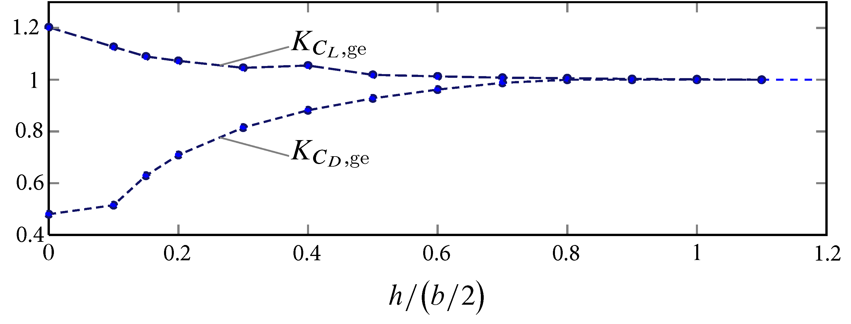
Plotted functions of non-dimensional ground altitude \(h/(b/2)\), defining the properties named 'aero/function/kCLge' and 'aero/function/kCDge' in the aerodynamic model of c172p.
Tables
One, two, or three dimensional lookup tables can be defined in JSBSim for use in aerodynamics and function definitions. For a single "vector" lookup table, the format is as follows:
<table name="property_name_0">
   <independentVar lookup="row"> property_name_1 </independentVar>
   <tableData>
      key_1  value_1
      key_2  value_2
      ...    ...
      key_n  value_n
   </tableData>
</table>
The lookup="row" attribute in the <independentVar/> element is optional in this case; it is assumed that the independentVar is a row variable. A real example is as shown here:
<table>
   <independentVar lookup="row"> aero/alpha-rad </independentVar>
   <tableData>
      -1.57  1.500
      -0.26  0.033
       0.00  0.025
       0.26  0.033
       1.57  1.500
   </tableData>
</table>
The first column in the data table represents the lookup index (or breakpoints, or keys). In this case, the lookup index is aero/alpha-rad (angle of attack in radians). If aero/alpha-rad is \(0.26\) radians, the value returned from the lookup table would be \(0.033\).
The definition for a 2D table, is as follows:
<table name="property_name_0">
   <independentVar lookup="row">    property_name_1 </independentVar>
   <independentVar lookup="column"> property_name_2 </independentVar>
   <tableData>
                  {col_1_key   col_2_key   ...  col_n_key }
      {row_1_key} {col_1_data  col_2_data  ...  col_n_data}
      {row_2_key} {...         ...         ...  ...       }
      {   ...   } {...         ...         ...  ...       }
      {row_n_key} {...         ...         ...  ...       }
   </tableData>
</table>
The data is in a gridded format. A real example is as shown below. Alpha in radians is the row lookup (alpha breakpoints are arranged in the first column) and flap position in degrees is split up in columns for deflections of 0, 10, 20, and 30 degrees):
<table>
   <independentVar lookup="row">    aero/alpha-rad   </independentVar>
   <independentVar lookup="column"> fcs/flap-pos-deg </independentVar>
   <tableData>
                 0.0          10.0        20.0       30.0
     -0.0523599  8.96747e-05  0.00231942  0.0059252  0.00835082
     -0.0349066  0.000313268  0.00567451  0.0108461  0.0140545
     -0.0174533  0.00201318   0.0105059   0.0172432  0.0212346
      0.0        0.0051894    0.0168137   0.0251167  0.0298909
      0.0174533  0.00993967   0.0247521   0.0346492  0.0402205
      0.0349066  0.0162201    0.0342207   0.0457119  0.0520802
      0.0523599  0.0240308    0.0452195   0.0583047  0.0654701
      0.0698132  0.0333717    0.0577485   0.0724278  0.0803902
      0.0872664  0.0442427    0.0718077   0.088081   0.0968405
  </tableData>
</table>
The definition for a 3D table in a coefficient would be (for example):
<table name="property_name_0">
   <independentVar lookup="row">    property_name_1 </independentVar>
   <independentVar lookup="column"> property_name_2 </independentVar>
   <independentVar lookup="table">  property_name_3 </independentVar>
   <tableData  breakpoint="table_1_key">
                  {col_1_key   col_2_key   ...  col_n_key }
      {row_1_key} {col_1_data  col_2_data  ...  col_n_data}
      {row_2_key} {...         ...         ...  ...       }
      {   ...   } {...         ...         ...  ...       }
      {row_n_key} {...         ...         ...  ...       }
   </tableData>
   <tableData  breakpoint="table_2_key">
                  {col_1_key   col_2_key   ...  col_n_key }
      {row_1_key} {col_1_data  col_2_data  ...  col_n_data}
      {row_2_key} {...         ...         ...  ...       }
      {   ...   } {...         ...         ...  ...       }
      {row_n_key} {...         ...         ...  ...       }
   </tableData>
   ...
   <tableData  breakpoint="table_n_key">
                  {col_1_key   col_2_key   ...  col_n_key }
      {row_1_key} {col_1_data  col_2_data  ...  col_n_data}
      {row_2_key} {...         ...         ...  ...       }
      {   ...   } {...         ...         ...  ...       }
      {row_n_key} {...         ...         ...  ...       }
   </tableData>
</table>
Note the breakpoint attribute in the tableData element, above. Here’s an example:
<table>
   <independentVar lookup="row">    fcs/row-value    </independentVar>
   <independentVar lookup="column"> fcs/column-value </independentVar>
   <independentVar lookup="table">  fcs/table-value  </independentVar>
   <tableData breakPoint="-1.0">
           -1.0    1.0
      0.0  1.0000  2.0000
      1.0  3.0000  4.0000
   </tableData>
   <tableData breakPoint="0.0000">
           0.0     10.0
      2.0  1.0000  2.0000
      3.0  3.0000  4.0000
   </tableData>
   <tableData breakPoint="1.0">
            0.0     10.0    20.0
       2.0  1.0000  2.0000  3.0000
       3.0  4.0000  5.0000  6.0000
      10.0  7.0000  8.0000  9.0000
   </tableData>
</table>
Note that table values are interpolated linearly, and no extrapolation is done at the table limits — the highest value a table will return is the highest value that is defined.
Interpolate 1D
Some lookup tables in simulation - particularly for aerodynamic data - can be four, five, six, or even more dimensional. Interpolate1d returns the result from a 1-dimensional interpolation of the supplied values, with the value of the first immediate child element representing the lookup value into the table, and the following pairs of values representing the independent and dependent values. The first provided child element is expected to be a property. The interpolation does not extrapolate, but holds the highest value if the provided lookup value goes outside of the provided range. The format is as follows:
<interpolate1d>
  {property, value, table, function}
  {property, value, table, function} {property, value, table, function}
  ...
</interpolate1d>
Example: If mach is 0.4, the interpolation will return 0.375. If mach is 1.5, the interpolation will return 0.60.
<interpolate1d>
  <p> velocities/mach </p>
  <v> 0.00 </v>  <v> 0.25 </v>
  <v> 0.80 </v>  <v> 0.50 </v>
  <v> 0.90 </v>  <v> 0.60 </v>
</interpolate1d>
The above example is very simplistic. A more involved example would use a function in any argument (except the first). That means that the breakpoint vector can be variable - which would probably not be common - but more importantly the values in the lookup vector (second column) could be function table elements of 1, 2, or 3 dimensions. The arguments could even be nested interpolate1d elements. For example:
<function name="whatever">
  <interpolate1d>
    <p> velocities/mach </p>
    <v> 0.00 </v>  <table> ... table definition ... </table>
    <v> 0.80 </v>  <table> ... table definition ... </table>
    <v> 0.90 </v>  <table> ... table definition ... </table>
  </interpolate1d>
</function>
Carrying this further:
<function name="bigWhatever1">
  <interpolate1d>
    <p> aero/qbar-psf </p>
    <v> 0 </v>  <interpolate1d>
                  <p> velocities/mach </p>
                  <v> 0.00 </v>  <table> ... table 1 definition ... </table>
                  <v> 0.80 </v>  <table> ... table 2 definition ... </table>
                  <v> 0.90 </v>  <table> ... table 3 definition ... </table>
                </interpolate1d>
    <v> 65 </v> <interpolate1d>
                  <p> velocities/mach </p>
                  <v> 0.00 </v>  <table> ... table 1 definition ... </table>
                  <v> 0.80 </v>  <table> ... table 2 definition ... </table>
                  <v> 0.90 </v>  <table> ... table 3 definition ... </table>
                </interpolate1d>
    <v> 90 </v> <interpolate1d>
                  <p> velocities/mach </p>
                  <v> 0.00 </v>  <table> ... table 1 definition ... </table>
                  <v> 0.80 </v>  <table> ... table 2 definition ... </table>
                  <v> 0.90 </v>  <table> ... table 3 definition ... </table>
                </interpolate1d>
  </interpolate1d>
</function>
The above effectively gives a five dimensional lookup table. It would be big and messy, in practice, but there it is. :-)
There is more, though. For very, very large aero databases there might be
times when some aero coefficients do not need to be calculated. For
instance, ground effects aero coefficients only need to be calculated close
to the ground. Why waste CPU cycles when the ground effects do not
contribute to the aero forces and moments? We can employ the ifthen element
to bypass expensive computations. The ifthen element works as follows:
If the value of the first immediate child element is 1, then the value of the second immediate child element is returned, otherwise the value of the third child element is returned.
If the value of the first immediate child element is 1, then the value of the second immediate child element is returned, otherwise the value of the third child element is returned.
<ifthen>
  {property, value, table, or other function element}
  {property, value, table, or other function element}
  {property, value, table, or other function element}
</ifthen>
Example: if flight-mode is greater than 2, then a value of 0.00 is returned, otherwise the value of the property control/pitch-lag is returned.
<ifthen>
  <gt> <p> executive/flight-mode </p> <v> 2 </v> </gt>
  <v> 0.00 </v>
  <p> control/pitch-lag </p>
</ifthen>
In our case, we could write the 5-dimensional table lookup as follows, returning a zero unless the gear is down:
<function name="propertyname">
  <ifthen>
    <lt> <p> position/altitudeMSL </p> <v> 90 </v> </lt>
    <interpolate1d>
      <p> aero/qbar-psf </p>
      <v> 0 </v>  <interpolate1d>
                    <p> velocities/mach </p>
                    <v> 0.00 </v>  <table> ... table 1 definition ... </table>
                    <v> 0.80 </v>  <table> ... table 2 definition ... </table>
                    <v> 0.90 </v>  <table> ... table 3 definition ... </table>
                  </interpolate1d>
      <v> 65 </v> <interpolate1d>
                    <p> velocities/mach </p>
                    <v> 0.00 </v>  <table> ... table 1 definition ... </table>
                    <v> 0.80 </v>  <table> ... table 2 definition ... </table>
                    <v> 0.90 </v>  <table> ... table 3 definition ... </table>
                  </interpolate1d>
      <v> 90 </v> <interpolate1d>
                    <p> velocities/mach </p>
                    <v> 0.00 </v>  <table> ... table 1 definition ... </table>
                    <v> 0.80 </v>  <table> ... table 2 definition ... </table>
                    <v> 0.90 </v>  <table> ... table 3 definition ... </table>
                  </interpolate1d>
    </interpolate1d>
    <v> 0 </v>
  </ifthen>
</function>
The above example is non-sensical in a way, but the format is correct. Performance-wise it is good because the tables do not get executed unless absolutely needed in the lookup.